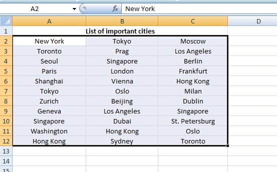
Select your data range (A2:C12)
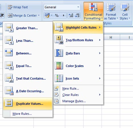
Click on Conditional Formatting (under Home tab) > then Highlight Cells Rules > click on Duplicate Values...
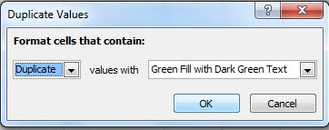
'Duplicate Values' window opens > select Duplicate from the drop down menu, and any color of your choice to highlight the duplicate cells > click OK.
Note: Here you could also select 'Unique' from the drop down list to highlight cells with unique values only. Try this as well
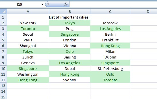
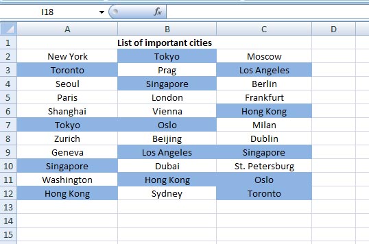
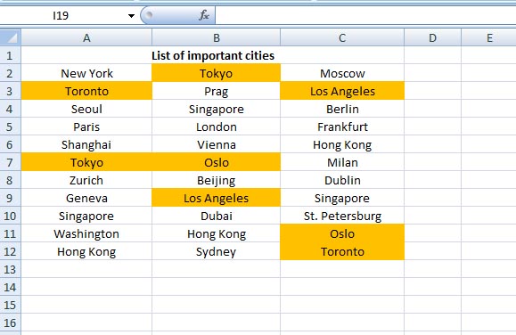
Values that are present more than once are now highlighted with your selected color. This includes duplicate entries as well as values present more than twice in the list.
Use a formula to get exactly the same result as above:
Select your data range (A2:C12)
Go to Conditional Formatting > this time click on New Rule...
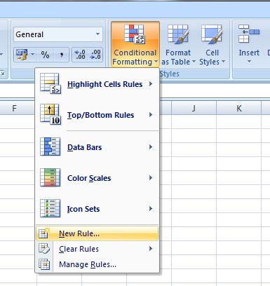
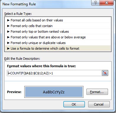
from the New Formatting Rule window > select Use a formula to determine which cells to format > here enter the formula =COUNTIF($A$2:$C$12;A2)>1
and from the Format... select any color to highlight the cells > click OK.
You have the same result as above, but this time you did it with a small programming
Few words on COUNTIF function:
COUNTIF function takes only two arguments - a range, and a criteria (it looks for the criteria within the range). So its syntax is
=COUNTIF(range, criteria)
So when I enter =COUNTIF($A$2:$C$12;A2)>1, the COUNTIF function looks for the criteria (cell A2 = New York) withn the range (A2:C12) and when it finds New York more than once(>1), it marks the cells containing New York with the blue color (that I selected under New Formatting Rule above).
As I have selected the range before clicking on Conditional Formatting, so the formula is copied automatically to other cells to look for the next entry and so on.
Look the interesting thing here:
In my list, Singapore and Hong Kong are present 3 times each. Here comes the point, you can now play with the Countif function
First select your cells (A2:C12) – don't forget it, (may be you do it in a new worksheet, just copy your original data)
then instead of =COUNTIF($A$2:$C$12;A2)>1 enter =COUNTIF($A$2:$C$12;A2)=2, it marks cells only with duplicates
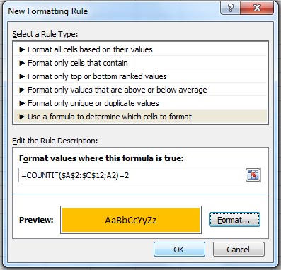
Result: only duplicate entries are highlighted.
Now to find values that are present more than two times:
instead of =COUNTIF($A$2:$C$12;A2)=2 enter =COUNTIF($A$2:$C$12;A2)>2
To find values present only 3 times:
instead of =COUNTIF($A$2:$C$12;A2)=2 enter =COUNTIF($A$2:$C$12;A2)=3
Don't forget to select your cells first!!
So now you know, how it works
*Recommended:
Read wonderful articles (English & German) on Science & Tech, Environment, Health and many other topics only on BlogArena.
For comments of suggestions, please contact us: info@shamskm.com