Its syntax is:
=ISBLANK(value)
In most cases, the 'value' argument is a cell reference.
Check the table below:
In cell B2 enter
=ISBLANK(A2)
Simply copy the formula down the column.
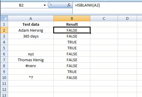
As you see, empty cells like A4 returns TRUE, while cells like A3 returns FALSE.
Now let's say, you don't want any text like those TRUE or FALSE for your spreadsheet, rather want to use any number like 0(Zero) for empty cells and 1(one) for not-empty cells.
For this case, I will use the ISBLANK Function within the IF function.
So enter in cell B2
=IF(ISBLANK(A2);0;1)
Copy this formula down the column.
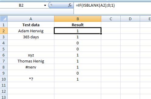
It says, if the given condition is met, that means if cell A2 is blank or empty, then put 0, otherwise put 1. That's it.
For those who want to learn the basics of IF function: read the tutorial here
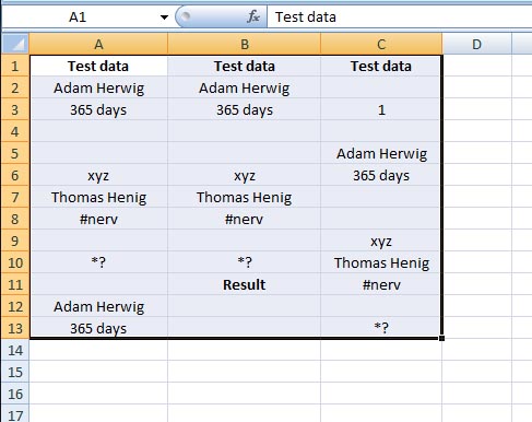
The two examples above show you in plain the use of ISBLANK function only. But in practical case, it's may be better to use the ISBLANK function with conditional formatting, to mark or highlight the blank cells with any color (to identify them easily). So let's start:
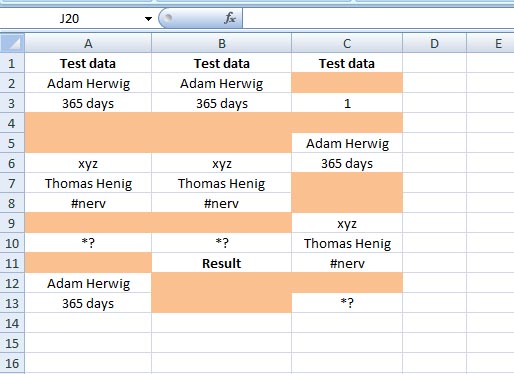
Select the cells (A1:C13)
Click on Conditional Formatting (you find it under the Home Tab) > Click on New Rule...
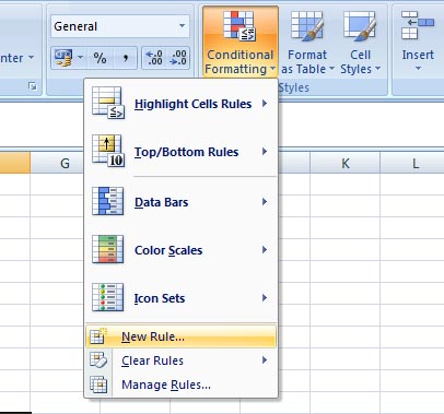
The New Formatting Rule window opens.
from Select a Rule Type > select Use a formula to determine which cells to format > here enter the formula =ISBLANK(A1)
and from the Format... select any color to highlight the blank cells > click OK.
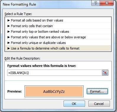
So how does the ISBLANK function works with the conditioanl formatting? First, it checks the cell A1 if the cell is empty (=ISBLANK(A1)), and if it finds the cell empty, then it highlights the cell with the selected color, otherwise it leaves the cell with its value. Now, as you have selected the whole range (A1:C13) before going to conditional formatting, it then looks for the next cell and format it if the condition is met, and so goes the story on.
Now you have the result:
Have fun