Create a Pareto Chart in Excel for Business Analysis
Posted: Wed Feb 01, 2017 11:28 am
Create a Pareto Chart in Excel for Business Analysis or Quality Control:
Pareto chart, named after the Italian economist Vilfredo Pareto, who noticed that 80% of Italy's land was owned by 20% of the population while at the University of Lausanne in 1896 . Hence comes the 80/20 rule.
So it can happen that, 80% of the unrest or problems you are facing in your factory or business comes from 20% of the workers or from 20% of the issues.
80% failure of the output or productivity is occurring from 20% of the issues.
Or something positve: 80% of your company's profit comes from 20% of customers.
80% of your company's revenue comes from 20% of its products.
So now you know how important is the Pareto Chart for quality control or for manegerial purposes.
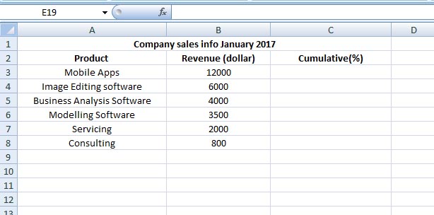
To create the Pareto Chart, the first thing you need to do: arrange your data in descending order.
In the example, I have arranged the revenue data in descending order in Column B. Now I will calculate cumulative percentage in Column C. May be you will need to format Column C to have the percentage format (click on the heading of Column C to select the whole column > right mouse click > click on Format Cells... > from Category choose Percentage, leave decimal places up to 2 > click OK).
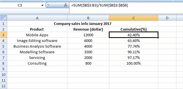
Now in cell C3 enter
=SUM($B$3:B3)/SUM($B$3:$B$8 )
Copy this down the column. Now you have the cumulative percentage.
So my data is ready now to start plotting the Pareto Chart.
Create the Chart:
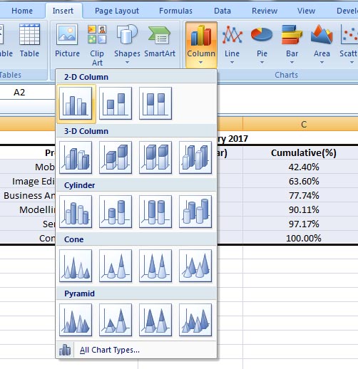
Select your data (A2:C8).
Go to Insert > Charts > here from 2-D Column select the first one (Clustered Column)
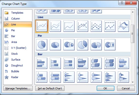
Now right click on the cumulative (%) bar from the legend > select Change Series Chart Type...
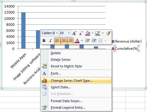
Change Chart Type window opens > from Line group select the first one > click OK.
The cumulative (%) bar is now changed to line > right click on it > click on Format Data Series...
The Format Data Series window opens. Here from Series Options click on Secondary Axis > click Close.
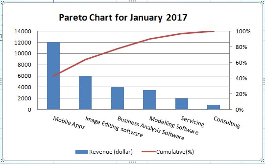
The Pareto Chart is ready so far. Now do the final polishing – like adjusting the values for the vertical axes (click on any of the axes > right mouse click > click on Format Axis.... > adjust the maximum and major unit values etc. as per your preference), giving a title to your chart (you can do the title from Chart Layouts that you will get under Design tab > select any layout of your choice )
)
Good work ahead guys
Read on Wikipedia: Pareto Principle
Pareto chart, named after the Italian economist Vilfredo Pareto, who noticed that 80% of Italy's land was owned by 20% of the population while at the University of Lausanne in 1896 . Hence comes the 80/20 rule.
So it can happen that, 80% of the unrest or problems you are facing in your factory or business comes from 20% of the workers or from 20% of the issues.
80% failure of the output or productivity is occurring from 20% of the issues.
Or something positve: 80% of your company's profit comes from 20% of customers.
80% of your company's revenue comes from 20% of its products.
So now you know how important is the Pareto Chart for quality control or for manegerial purposes.
To create the Pareto Chart, the first thing you need to do: arrange your data in descending order.
In the example, I have arranged the revenue data in descending order in Column B. Now I will calculate cumulative percentage in Column C. May be you will need to format Column C to have the percentage format (click on the heading of Column C to select the whole column > right mouse click > click on Format Cells... > from Category choose Percentage, leave decimal places up to 2 > click OK).
Now in cell C3 enter
=SUM($B$3:B3)/SUM($B$3:$B$8 )
Copy this down the column. Now you have the cumulative percentage.
So my data is ready now to start plotting the Pareto Chart.
Create the Chart:
Select your data (A2:C8).
Go to Insert > Charts > here from 2-D Column select the first one (Clustered Column)
Now right click on the cumulative (%) bar from the legend > select Change Series Chart Type...
Change Chart Type window opens > from Line group select the first one > click OK.
The cumulative (%) bar is now changed to line > right click on it > click on Format Data Series...
The Format Data Series window opens. Here from Series Options click on Secondary Axis > click Close.
The Pareto Chart is ready so far. Now do the final polishing – like adjusting the values for the vertical axes (click on any of the axes > right mouse click > click on Format Axis.... > adjust the maximum and major unit values etc. as per your preference), giving a title to your chart (you can do the title from Chart Layouts that you will get under Design tab > select any layout of your choice
Good work ahead guys
Read on Wikipedia: Pareto Principle