The SUMIF function accepts only one criteria or conditon at a time, while as the name says, SUMIFS function accepts multiple conditions or criteria. So the SUMIFS function offers more flexibilty for data analysis.
The syntax of SUMIF function:
=SUMIF(range, criteria, [sum_range])
The syntax for SUMIFS function:
=SUMIFS(sum_range, criteria_range1, criteria1, [criteria_range2, criteria2], ...)
sum_range is a required field. It specifies the range of cells that are to be added up.
criteria_range1 is the first range of cells where the first criteria (criteria1) is to be evaluated. It's a required field.
criteria1 is the condition that is to be evaluated in the criteria_range1. It's a required field.
So how it works?
The condition you put as criteria1 is searched within the range of cells given as criteria_range1 and if found, then their corresponding values are summed up from the sum_range.
criteria_range2, criteria2 are the next range of cells with the respective criteria or conditions. These are optional. The SUMIFS function can take upto a total of 127 range/criteria pairs.
Let's try the following example:
In the following table, I have data of sales agents, items they sell and pieces they sold.
First, I want to calculate total pieces of iPhone sold by sales agent Adam? So in cell C16 enter
=SUMIFS(C2:C13;B2:B13;"iPhone";A2:A13;"Adam")
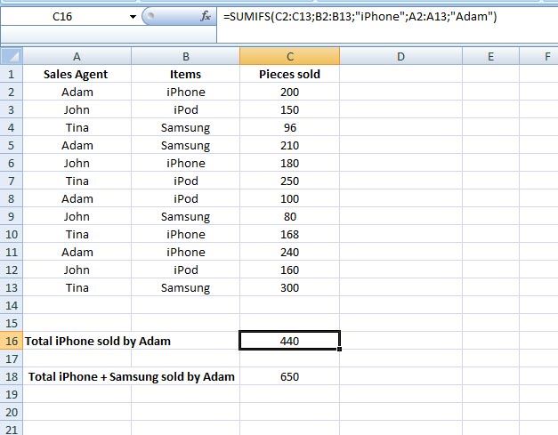
Result: 440
Here, C2:C13 is my sum_range
B2:B13 is my criteria_range1
"iPhone" is my criteria1 or my first condition
A2:A13 is my criteria_range2
"Adam" is my criteria2 or my second condition
Now, let's say I would like to calculate total peices of iPhone + Samsung sold by Adam. For this I will use the SUMIFS function within the SUM function. So let's enter in cell C18:
=SUM(SUMIFS(C2:C13;B2:B13;{"iPhone";"Samsung"};A2:A13;"Adam"))
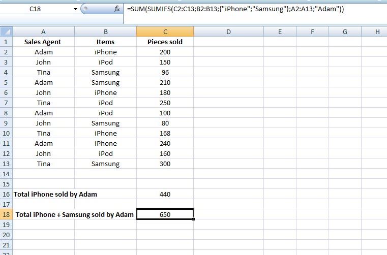
Result: 650
Explanation is as above. The only thing is, here criteria1 contains two text strings. They are within the curly brackets and separated by semi-colon – {"iPhone";"Samsung"}.
Thus if Adam and Tina would be your criteria2, then type – {"Adam";"Tina"}
This way, you could have multiple text strings in each criteria.
Have fun