Its syntax is very simple with only one argument
=ISERROR(value)
Most cases, the 'value' argument is a cell reference.
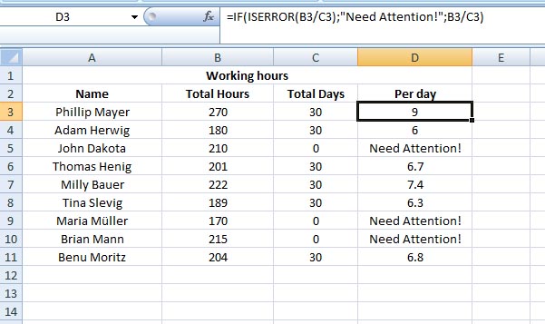
In the following example, I will calculate per day working hour in Column D. For me, it's more practical to use the ISERROR function inside an IF function, so that if there occurs an error in the calculation, I can see the cells for further corrections with a friendly notice rather than those nerve-taking typical error warnings like #DIV/0! or #NUM!, so to say.
So in cell D3 enter
=IF(ISERROR(B3/C3);"Need Attention!";B3/C3)
Copy the formula down the column – you can see the cells that nee your attention!!
Let's try something different:
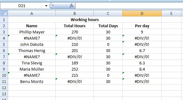
Let's say, your colleague sent you an Excel sheet full of calculations with plenty of errors, and you would like to mark those erro cells before you proceed to rework on the file.
Select the whole sheet (Ctrl + A)
Go to Conditional Formatting (under Home tab) > click on New Rule...
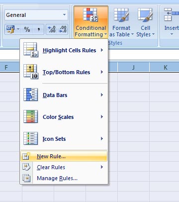
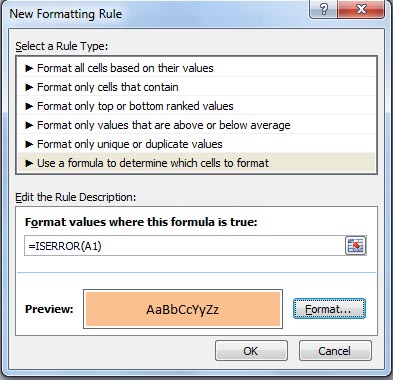
The New Formatting Rule window opens > select Use a formula to determine which cells to format.
Enter the following formula in the field under Edit the Rule Description:
=ISERROR(A1)
From the Format... button select any color to highlight the error cells > click OK.
The result is as follows:
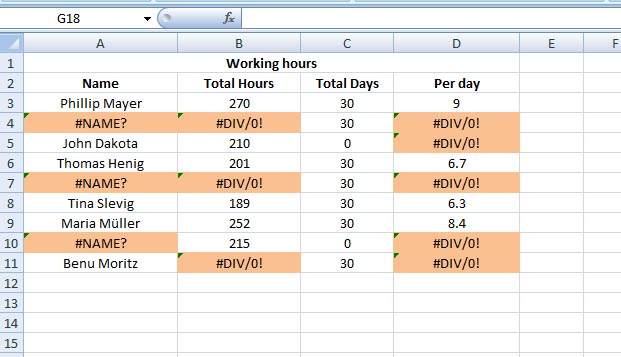
Good work ahead